Probability & Statistics in Engineering
Fall 2023 - 30 Nov


 https://aerossurance.com/safety-management/challenger-launch-decision-30/
Empirical models
- Relationship between two or more variables
- Pressure of a gas in a container related to temperature
- Water velocity in open channel related to width
- Regression analysis
- One independent variable \(X\) and one dependent \(Y\) with a linear relationship
- \(Y=\beta_0 + \beta_1 x_1 + ... + \beta_r x_r\)
- \(Y=\beta_0 + \beta_1 x_1 + ... + \beta_r x_r + \epsilon\)
Example
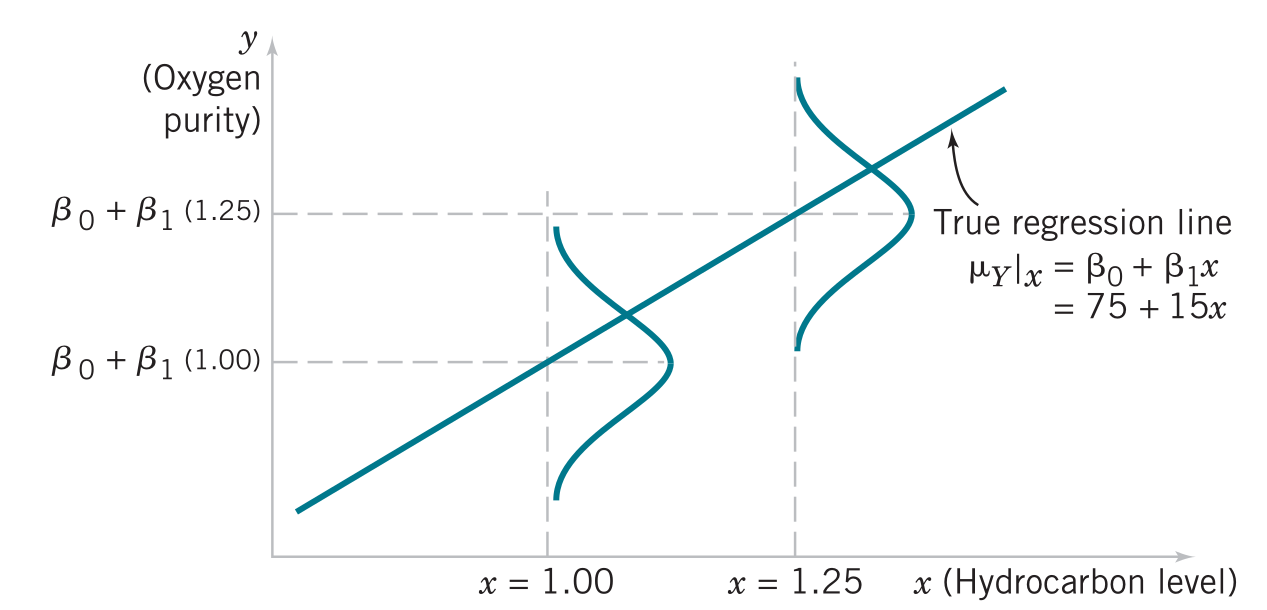
Simple linear regression model
\[E[Y|x]=\mu_{Y|x}=\alpha + \beta x\]
\(\alpha\): intercept and \(\beta\): slope are the regression coefficients
\[Y=\alpha + \beta x + \epsilon\] is the simple linear regression model
\[E[Y|x]=E[\alpha+\beta x+\epsilon]=\alpha+\beta x+E[\epsilon]=\alpha+\beta x\]
\[\text{Var}(Y|x)=\text{Var}(\alpha+\beta x+\epsilon)=\text{Var}(\alpha+\beta x)+\text{Var}(\epsilon)=0+\sigma^2=\sigma^2\]
Estimating the regression coefficients
\[Y = \alpha + \beta x + \epsilon\]
\(\epsilon\) are assumed to be uncorrelated random errors with mean zero and unknown variance \(\sigma^2\)
\(n\) pairs of observations \((x_1, y_1)\), \((x_2, y_2)\),…, \((x_n, y_n)\)
\[y_i=\alpha + \beta x_i + \epsilon_{i}\]
Least squares
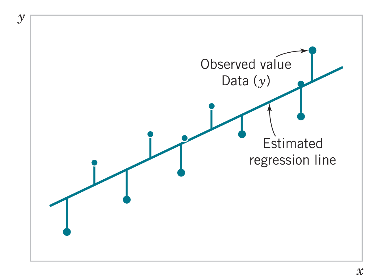
Minimize the sum of squares of the vertical deviations (method of least squares)
\[L = \sum_{i=1}^{n} \epsilon_{i}^{2} = \sum_{i=1}^n (y_i - \alpha - b x_i)^2\]
\[ \frac{\partial L}{\partial \alpha} = -2 \sum_{i=1}^n \left( y_i-A-B x_i \right) = 0\]
\[\dfrac{\partial L}{\partial \beta} = -2 \sum_{i=1}^n \left( y_i-A - B x_i \right)x_i = 0\]
The least squares estimates of the slope and intercept are \[A = \overline{y} - B \overline{x}\] \[B=\dfrac{\sum_{i=1}^n x_i y_i - \overline{x} \sum_{i=1}^n y_i}{\sum_{i=1}^n x_i^2 - n \overline{x}^2}\] where \(\overline{x}=(1/n)\sum_{i=1}^n x_i\) and \(\overline{y}=(1/n) \sum_{i=1}^n y_i\)
The estimated regression line is therefore \[\hat{y}=A + B x\] and each observation pair satisfies \[y_i=A+B x_i +e_i\] where \(e_i=y_i-\hat{y}_i\) is the residual
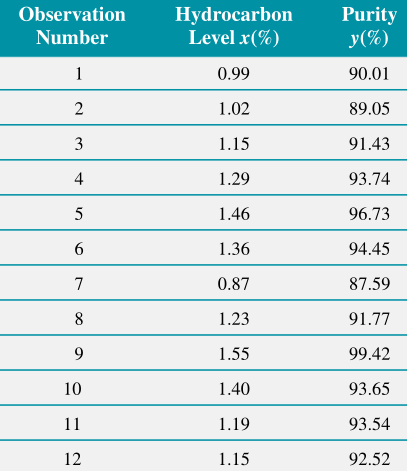
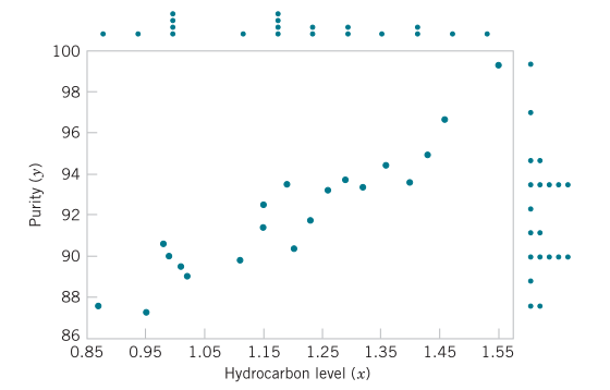
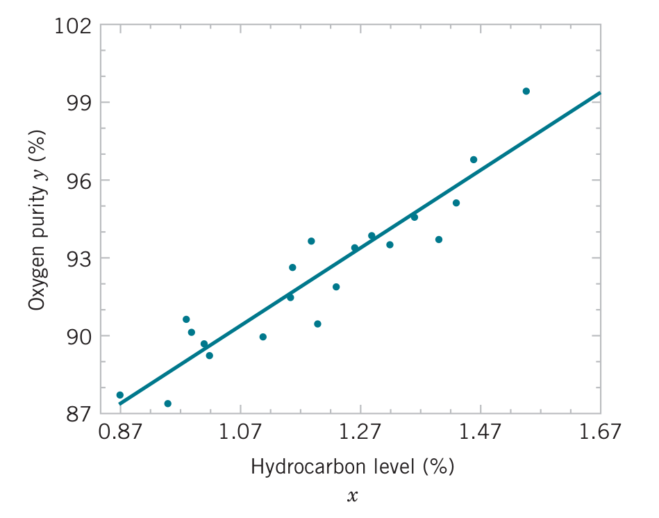
Example
Fit a simple linear regression model to the oxygen purity data. From calculations of the \(n=20\) observations we have \(\sum x_i=23.92\), \(\sum y_i=1843.21\), \(\overline{x}=1.1960\), \(\overline{y}=92.1605\), \(\sum y_i^2=170044.5321\), \(\sum x_i^2=29.2892\), and \(\sum x_iy_i=2214.6566\).
Alternative notation
\[S_{xy} = \sum_{i=1}^n (x_i - \overline{x})(y_i - \overline{y}) = \sum_{i=1}^n x_i y_i - n \overline{x} \overline{y}\]
\[S_{xx} = \sum_{i=1}^n (x_i - \overline{x})^2 = \sum_{i=1}^n x_i^2 - n \overline{x}^2\]
\[S_{yy} = \sum_{i=1}^n (y_i - \overline{y})^2 = \sum_{i=1}^n y_i^2 - n \overline{y}^2\]
\[B = \dfrac{S_{xy}}{S_{xx}}\] \[A = \overline{y} - B \overline{x}\]
Estimating \(\sigma^2\)
\[{SS}_E = \sum_{i=1}^n e_i^2 = \sum_{i=1}^n (y_i-\hat{y}_i)^2\]
\[{SS}_E = {SS}_T - B S_{xy}\] \[{SS}_T=\sum_{i=1}^n (y_i-\overline{y})^2 = \sum_{i=1}^n y_i^2 - n\overline{y}^2\]
\[\hat{\sigma}^2 = \dfrac{{SS}_E}{n-2}\]
Properties of least squares estimators
\[E[B] = B\] \[\text{Var}(B) = \dfrac{\sigma^2}{S_{xx}}\] \[E[A]=A\] \[\text{Var}(A) = \sigma^2 \left( \dfrac{1}{n} + \dfrac{\overline{x}^2}{S_{xx}} \right)\]
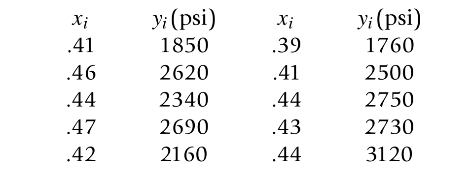
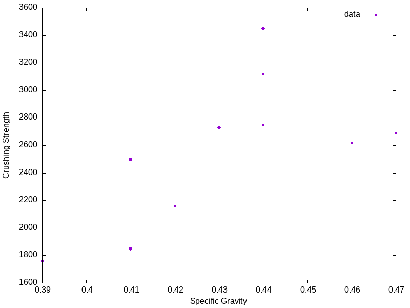
Problem 21.1
The following data describe specific gravity \(x\) of a wood sample and its maximum crushing strength \(y\):
| x | y |
|---|---|
| .41 | 1850 |
| .46 | 2620 |
| .44 | 3450 |
| .47 | 2690 |
| .42 | 2160 |
| .39 | 1760 |
| .41 | 2500 |
| .44 | 2750 |
| .43 | 2730 |
| .44 | 3120 |
Plot a scatter diagram. Does a linear relationship seem reasonable?
Estimate the regression coefficients.
Predict the maximum crushing strength of a wood sample whose specific gravity is 0.43