Probability & Statistics in Engineering
Fall 2023 - 14 Nov
Interval estimates
- Suppose that \(X_1\), \(X_2\),…, \(X_n\) is a sample of a normal population that has mean \(\mu\) and \(\sigma^2\)
- The MLE estimate of \(\mu\) is \(\overline{X}=\sum_{i=1}^n X_i / n\)
- We don't expect \(\overline{X}\) to be exactly equal to \(\mu\)
- But it should be close
- Rather than a point estimate we can specify an interval
- We can assign a degree of confidence that \(\mu\) lies within that interval
- The distribution of the point estimator can be used to obtain the interval estimator
Confidence intervals
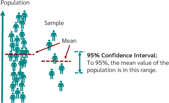
- An interval estimate for a population parameter
- Usually they are 90%, 95% and 99%
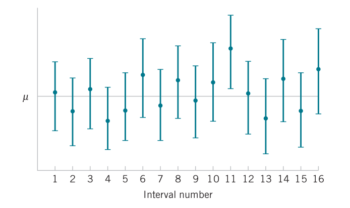
- Measure of reliability: if we repeated the experiment multiple times and calculated the 95% bounds then 95% of samples would contain the true mean within their corresponding bounds
- Confidence interval for mean, variance and proportion
- Cases of normal distribution with known or unknown variance
The 95% confidence interval on the mean

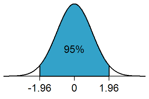
Remember that \(\dfrac{\overline{X}-\mu}{\sigma / \sqrt{n}}\) is a standard normal variable

\[P \left( -1.96 < \dfrac{\overline{X}-\mu}{\sigma / \sqrt{n}} < 1.96 \right) = 0.95\]
\[P \left( -1.96 \dfrac{\sigma}{\sqrt{n}} < \overline{X}-\mu < 1.96 \dfrac{\sigma}{\sqrt{n}} \right) = 0.95\]
\[P \left( -1.96 \dfrac{\sigma}{\sqrt{n}} < \mu - \overline{X} < 1.96 \dfrac{\sigma}{\sqrt{n}} \right) = 0.95\]
\[P \left( \overline{X} - 1.96 \dfrac{\sigma}{\sqrt{n}} < \mu < \overline{X} + 1.96 \dfrac{\sigma}{\sqrt{n}} \right) = 0.95\]
With 95% confidence, the true mean lies within \(1.96 \dfrac{\sigma}{\sqrt{n}}\) of the sample mean and the 95 percent confidence interval is \[\left(\overline{X} - 1.96 \dfrac{\sigma}{\sqrt{n}}, \overline{X} + 1.96 \dfrac{\sigma}{\sqrt{n}} \right)\]
Problem 17.1
The amplitude of a signal received is random variable due to noise during transmission, but it follows a distribution \(\text{N}(\mu, 4)\). If the amplitudes measured 9 times are 5, 8.5, 12, 15, 7, 9, 7.5, 6.5, 10.5 what is the 95% confidence interval for the true amplitude \(\mu\)?
Two-sided and one-sided intervals
What if we were interested in \(\mu\) being at least as large as value (relative to the mean)?
\[P(Z < 1.645) = 0.95 \Rightarrow P \left( \dfrac{\overline{X}-\mu}{\sigma / \sqrt{n}} < 1.645 \right) = 0.95\]
\[P \left( \overline{X} - 1.645 \dfrac{\sigma}{\sqrt{n}} < \mu \right) = 0.95\]
One-sided upper 95% confidence interval \[\left( \overline{X} - 1.645 \dfrac{\sigma}{\sqrt{n}}, \infty \right)\] One-sided lower 95% confidence interval \[\left(-\infty, \overline{X} + 1.645 \dfrac{\sigma}{\sqrt{n}} \right)\]
Problem 17.2
Find the upper and lower 95% confidence intervals from the previous example.
Confidence intervals of any specified level

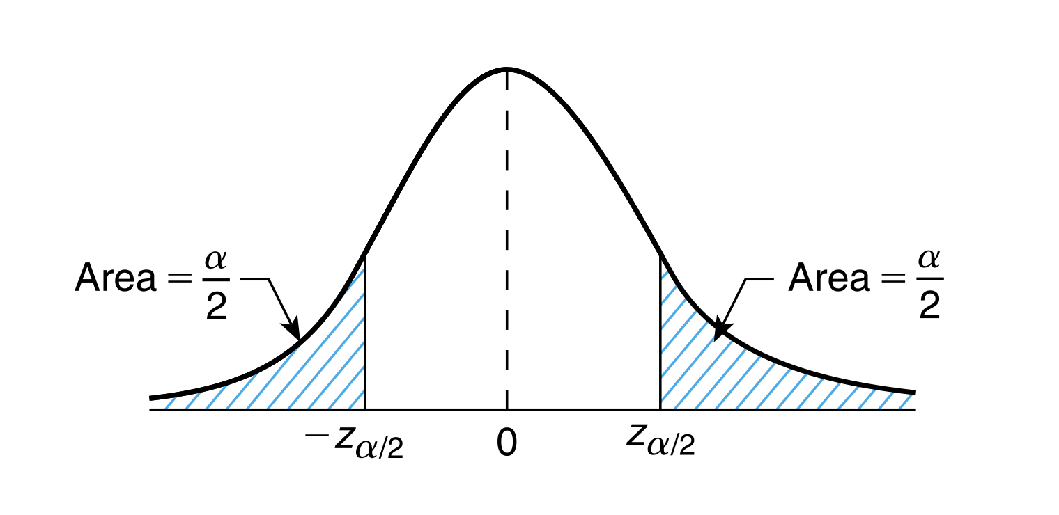
\[P(Z > z_a) = a\]
\[P \left( -z_{a/2} < Z < z_{a/2} \right) = 1-a \Rightarrow P \left( -z_{a/2} < \dfrac{\overline{X}-\mu}{\sigma / \sqrt{n}} < z_{a/2} \right)\]
\[P \left( \overline{X} - z_{a/2} \dfrac{\sigma}{\sqrt{n}} < \mu < \overline{X} + z_{a/2} \dfrac{\sigma}{\sqrt{n}} \right)\]
The \(100(1-a)\) percent two-sided confidence interval for \(\mu\) is \[\left( \overline{X} - z_{a/2} \dfrac{\sigma}{\sqrt{n}}, \overline{X} + z_{a/2} \dfrac{\sigma}{\sqrt{n}} \right)\]
The \(100(1-a)\) percent one-sided lower confidence interval for \(\mu\) is \[\left( -\infty, \overline{X} + z_{a} \dfrac{\sigma}{\sqrt{n}} \right)\] The \(100(1-a)\) percent one-sided upper confidence interval for \(\mu\) is \[\left( \overline{X} - z_{a} \dfrac{\sigma}{\sqrt{n}}, \infty \right)\]
Problem 17.3
Use the previous data to calculate the 99% confidence intervals (both two- and one-sided).
Choosing the sample size
- Ten measurements of impact energy on specimens of steel materials had a mean of 64.46 J
- Impact energy is normally distributed with \(\sigma=1\) J
- How many steel material specimens do we need to keep the 99% bounds at most 1.0 J?

\[\left( \overline{X} - 2.58 \dfrac{\sigma}{\sqrt{n}}, \overline{X} + 2.58 \dfrac{\sigma}{\sqrt{n}} \right)\]
The interval length is \[5.16 \dfrac{\sigma}{\sqrt{n}}\]
\[n = (51.6 \sigma)^2 = 51.6 \approx 52\]
If \(\overline{x}\) is used as an estimate of \(\mu\), we can be \(100(1-a)%\) confident that the error \(|\overline{x}-\mu|\) will not exceed \(E\) when the sample size is \[n=\left( \dfrac{z_{a/2}\sigma}{E} \right)^2\]
Interpreting a confidence interval
- Probability of \(\mu\) being within the CI we calculated?
- Subtle difference between probability and confidence
- The CI is itself a random interval

Problem 17.4
The average speed of vehicles on a highway is being studied. Observations on 50 vehicles yielded a mean of 65 mph. Assume that the standard deviation is known to be 6 mph. What is the 2-sided 99% confidence interval on the mean speed?
How many additional vehicles need to be observed so that the mean speed can be estimated within \(\pm 1\) mph with 99% confidence?
If two engineers collect data and each one separately observes 10 vehicles, what is the probability that Engineer 1 will have a sample mean larger than Engineer's 2 by 2 mph?
What if the two engineers observed 100 vehicles instead?