Probability & Statistics in Engineering
Fall 2023 - 26 Oct
Bell curve
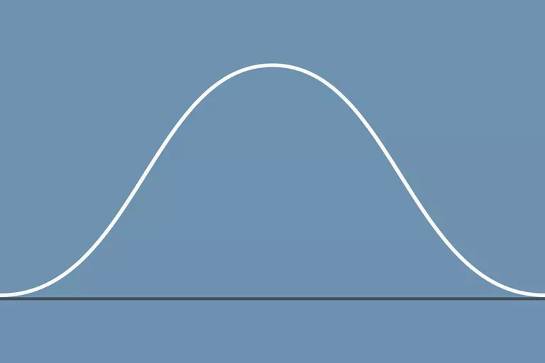

Normal distribution
A random variable \(X\) with probability density function
\[f(x)=\dfrac{1}{\sqrt{2 \pi} \sigma} e^{-\dfrac{(x-\mu)^2}{2\sigma^2}}\] is a normal random variable with parameters \(\mu\) and \(\sigma\)
The notation \(N(\mu,\sigma^2)\) is used for the normal distribution, with \(E[X]=\mu\) and \(\text{Var}(X)=\sigma^2\)
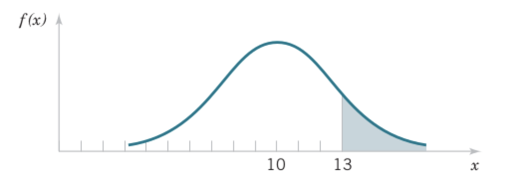
Example
Measurements of current in a strip of wire follow a normal distribution \(N(10,4)\). What is the probability that a measurement exceeds 13 mA?
Probabilities of a normal distribution
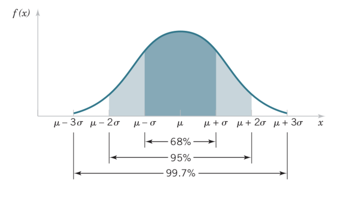
\[P(\mu-\sigma < X < \mu+\sigma)=0.6827\] \[P(\mu-2\sigma < X < \mu+2\sigma)=0.9545\] \[P(\mu-3\sigma < X < \mu+3\sigma)=0.9973\] \[P(X<\mu)=P(X>\mu)=0.5\]
Standard normal distribution
A normal random variable with \[\mu=0 \text{ and } \sigma^2=1\] is called a standard normal random variable, denoted as \(Z\).
The cumulative distribution function of a standard normal random variable is \[\Phi(z) = P(Z \leq z)\]
Standard normal CDF
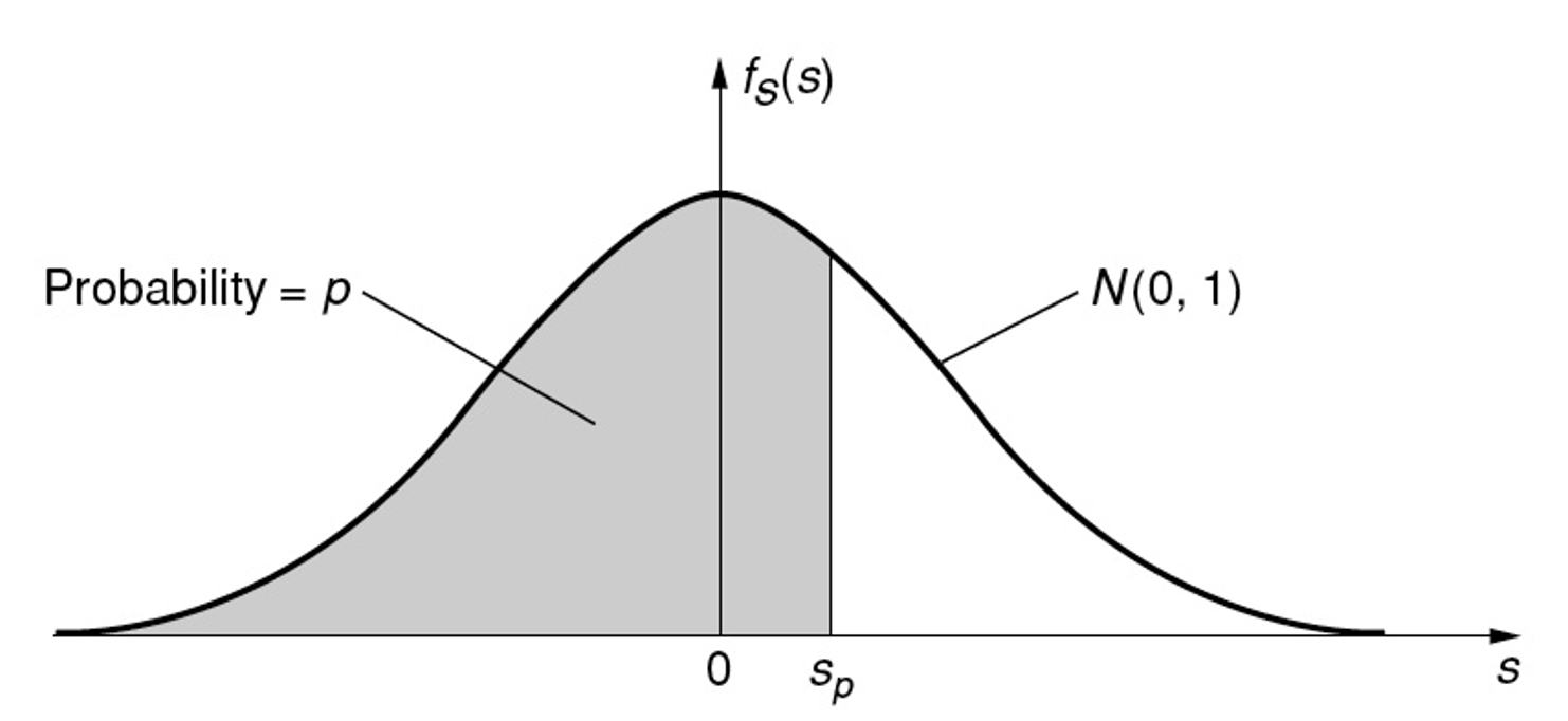
\[s_p = \Phi^{-1}(p)\]
Tables
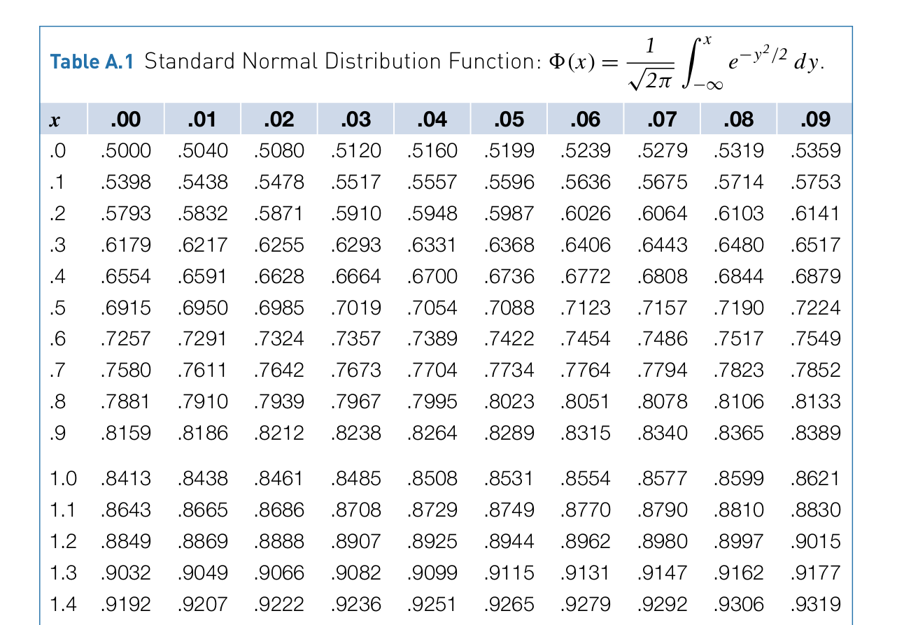
\[\Phi(-z)=1-\Phi(z)\] \[z=\Phi^{-1}(p)=-\Phi^{-1}(1-p)\]
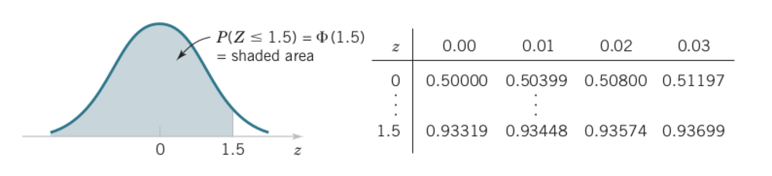
Example
Let's find \(P(Z \leq 1.5)\) and \(P(Z \leq 1.53)\)
Your turn!
- \(P(Z > 1.15)\)?
- \(P(Z < -0.77)\)?
- \(P(-1.25 < Z < 1.37)\)?
- \(P(Z \leq -4.6)\)?
- \(z\) when \(P(Z>z)=0.05\)?

Standardizing a normal random variable
If \(X\) is a normal random variable with \(E[X]=\mu\) and \(V(x)=\sigma^2\), the random variable \[Z=\dfrac{X-\mu}{\sigma}\] is a normal random variable with \(E[Z]=0\) and \(\text{Var}(Z)=1\).
Standardizing to calculate a probability
Suppose that \(X\) is a random variable with mean \(\mu\) and variance \(\sigma^2\).
\[P(X \leq x) = P \left( \dfrac{X-\mu}{\sigma} \leq \dfrac{x-\mu}{\sigma} \right) = P(Z \leq z)\]
where \(Z\) is a standard normal variable, and \(z=\dfrac{x-\mu}{\sigma}\).
Problem 12.1
Drainage from a community during a storm is a normal variable with a mean of 1.2 mgd and a standard deviation of 0.4 mgd. If the storm drain is designed with a maximum capacity of 1.5 mgd, what is the underlying probability of flooding during a storm that is assumed in the design of the drainage system?
Problem 12.2
Statistical data show that the annual vehicle miles driven between traffic accidents is a normal random variable with mean 15,000 miles/year and a coefficient of variation of 25%. What is the probability of someone who drives 10,000 miles to have an accident in a year?
If the same driver has already driven 8,000 miles, what is the probability of them having an accident for the remainder of that year?
Problem 12.3
Specifications for the fabrication of steel beams require that the actual lengths be within \(\pm5 \text{ mm}\) of the specified dimensions with a probability (i.e., reliability) of 99.7%. What is the required precision in terms of an allowable \(\sigma\), assuming a non-biased production process?